While articles like this aren’t going to be the focus of what we do, we are hoping to have the occasional piece that try to take some simple, yet hard-to-answer questions about the NFL and look to investigate them from a more data-driven perspective. We hope that this will allow for some insight into how data can be used in sports more generally, not just the NFL, and maybe even come up with a useful new metric of our own every now and then. More importantly though, we think this is an opportunity to give you more information about the game and allow you to feel a little smarter when talking about the game with your friends.
Welcome to “Beyond the Numbers”.
The NFL Combine has long been an important fixture in the NFL calendar, and coming in the natural lull of interest following the Super Bowl, it has naturally attracted an increasing level of media attention in recent years. Never before has the importance of a wide receiver’s 40 or the fluidity with which a cornerback flips his hips been more significant in the mind of the NFL fan. While the 2021 NFL Combine will not look like that of recent seasons due to the ongoing COVID pandemic, teams will still be able to collect athletic data at pro days and while it might not be in a format as easy to digest for fans as the Combine, the role of athletic data in the scouting process will likely remain unchanged.
But just how important is the Combine?
It’s easy to point to the players who have had very successful NFL careers despite poor athletic measurables; Anquan Boldin’s 4.71 40 yard dash springs to mind; Panthers fans should be all-too-familiar with Dave Gettleman’s view of “I don’t care what a guy runs on a watch in his underwear.” Others will furiously espouse the predictive capabilities of the Combine, retweeting a grainy screenshot of an Excel spreadsheet that allegedly proves that if an edge rusher has a subpar 3 cone time they are guaranteed to be a bust.
Given the role that athletic measurables have played in the scouting process of the Seahawks, where new Panthers’ GM Scott Fritterer has been hired from, it seems worthwhile to see whether this focus on athletic measurables is something they can continue to push compared to the rest of the NFL in order to gain an edge, or whether by doing so, they will in fact be over-valuing such data.
In short — would overvaluing athletic measurables be a bad decision?
What I’ve Actually Done
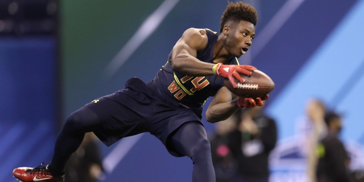
Photo: AP/David J. Phillip
The basic idea is to see if Combine data could predict how good an NFL player a prospect becomes. This is essentially predictive statistics: given some independent input variables, generate a model that can accurately predict this dependent variable. In this case the independent input variables are any Combine data (40 yard time, weight, 3 cone time, etc.), and the dependent variable is this nebulous idea of how good an NFL player is.
For the independent input variables, Combine data is readily accessible from Pro Football Reference with data files such as this dating back to 2000. Finding a manageable dependent variable to work with is less simple.
Given that we want to look at every position possible, one universal metric is Pro Football Reference’s AV. This is essentially an estimate of a player’s value in a given season. It’s not perfect as a metric, but provides a reasonable enough metric to use here. For example, taking a look at the Career AV accumulated by the 2011 NFL Draft, the top 6 players are Cam Newton, JJ Watt, Von Miller, Julio Jones, Richard Sherman and Patrick Peterson. The only caveat to this is that because so few quarterbacks and special teamers opt to take part in Combine drills, I have decided not to include them in this analysis as the data sets are too incomplete.
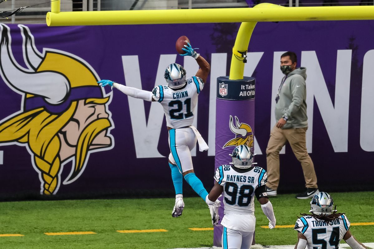
Photo Credit: Brace Hemmelgarn/USA TODAY Sports
The next decision to make was in what way to use the AV. One option was to use the career AV accumulated by each player, but this runs the risk of overvaluing longevity compared to production and while longevity is important, this is ultimately not what we are trying to measure. Additionally, career AV makes it hard to compare active and retired players on equal footing and so a further compromise is required.
The compromise was to use the sum of the AV from the players first 5 seasons. This allows the inclusion of all draft classes up to and including the 2016 NFL draft. The first five years of a player’s career should provide a good indication of their talent and offers a good compromise between the accuracy achieved through averaging and the size of the dataset. The one notable drawback to this method was that if a player had an injury riddled first five seasons, their AV wouldn’t correctly indicate their talent.
Given the size of the data set (1973 players), however, this should only be a minor effect.
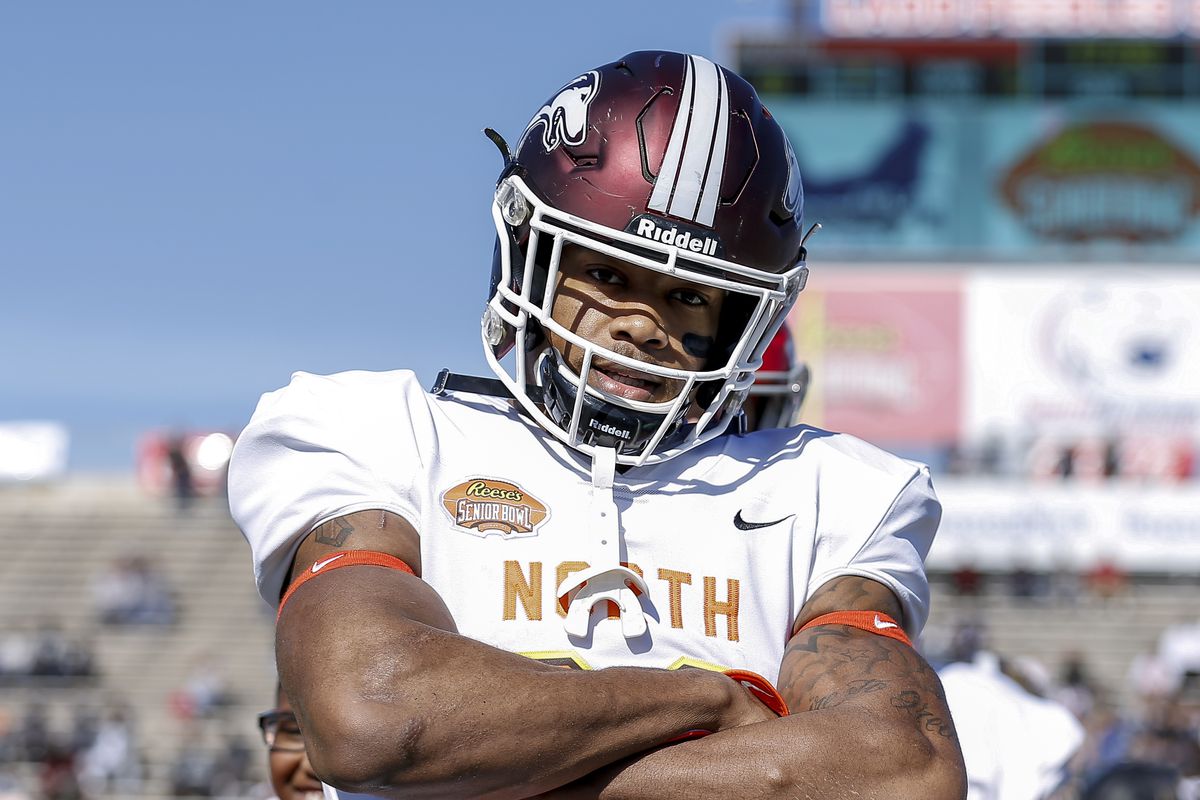
Photo Credit: Don Juan Moore/Getty Images
It is worth mentioning at this point that it is not important to understand how these models work in order to understand the takeaway of the information they provide. If this is not your thing, please feel free to skip over these sections, they are merely included for those who might be interested and to provide a record of what has actually been done for anybody who might want to try and either replicate this work or build upon it.
The model itself uses a multivariate linear regression; essentially the computer assumes that if it multiplies the different inputs by the right weightings and then adds them together it will get the correct output. The larger the weighting, the more important that independent variable is in determining the result. The computer then brute-forces it’s way to the best set of weightings, by changing them a little, looking at how close the predictions are to the real thing, and repeating until it can make no more improvements.
This is essentially like trying to learn to cook by taking a set of ingredients and trying them in different quantities until you get the best possible meal. While we would suggest that you stick to a recipe when you make your dinner later, in the case of Combine data, no recipes exist and so this is the best that we have to work with.

Linear regressions may be simple (at least with respect to other models), but they generally give good results, and are also useful for an important reason; the model is completely transparent. You can look at the set of weightings (hereafter referred to as coefficients), to see how important a variable is. This therefore not only allows for the testing the predictive capabilities of Combine data, but also allows us to see which drills are particularly important for a given position.
For a bit of fun, I also decided to see if Support Vector Machines would give better results than the simple linear regression. Support Vector Machines are a basic form of machine learning – using some principles of linear algebra and a lot of testing data the computer comes up with a predictive model. The downside to Support Vector Machines is that they are a bit of a black box, as there is no analogous set of coefficients you can use to try and understand the model.
Some additional points before we look at the results: the data was segmented based on position, and the pick a player was drafted at was also included as an independent variable. The addition of pick was a way to give an insight into the NFL’s evaluation of a player. This isn’t truly an independent variable, as NFL front offices select players partially based on their Combine data, but the inclusion of this will be explained more fully later on. More details on the methodology are given at the bottom of the article for those who are interested, but no greater understanding is necessary to understand the results.
What Can The Models Predict?

The data below is presented in three different forms; weighting coefficients for the different input variables, R^2 values for the linear regression model and R*2 values for the support vector machine model (which we have labelled SVR R^2 for the sake of clarity). Again, please feel free to skip the tables and focus on the conclusions drawn from them, but we have included the tables here for those who are interested.
Weighting coefficients are the values with which the inputs are multiplied in order to adjust for their relative importance. Here, the weighting coefficients presented have been normalized, meaning that the values for different drills and different positions can be compared directly. A positive value means that performance in this drills correlates with NFL success, whereas a negative value indicates that players who perform badly in this drill actually have better NFL careers, with the larger the value (positive or negative) the stronger the predictive value of this drill.

The R^2 value evaluates how good the model is as predicting the dependent variable. “R^2” is the result for the linear regression, and “SVR R^2” is the result for the support vector machine model. It’s possible values range from 1 to -1 with an R^2 of 1 indicates that the model is perfect at making predictions (however in this case you’ve probably overfitted the data). An R^2 of 0 indicates that the model is no better than random at predicting the dependent variable and an R^2 of -1 indicates that the model is worse than random at predicting the dependent variable
Firstly, let’s look at the predictive value of the pick with which a player was selected. This is essentially a test of how good the NFL as a whole is at evaluating different positions. For the sake of clarity, bigger values for the pick mean that this is more important, and the more positive the R^2 and SVR R^2 values, the better the model was able to predict the player outcomes based on the input data:
| Pos | Pick | R^2 | SVR R^2 |
|---|---|---|---|
| RB | 0 | -0.01 | -0.01 |
| WR | 0.42 | 0.27 | 0.25 |
| TE | 0.58 | 0.14 | 0.18 |
| OL | 0 | 0 | 0 |
| DL | 0.54 | 0.24 | 0.28 |
| Edge | 0 | -0.01 | -0.01 |
| LB | 0.58 | 0.3 | 0.37 |
| S | 0.06 | -0.02 | -0.01 |
| CB | 0.43 | 0.24 | 0.32 |
From this, it should be clear that the NFL is much better at predicting some positions than others.
Running backs, offensive linemen, edge rushers and safeties all show no meaningful correlation with where they were selected. Conversely, receivers, tight ends, interior defensive linemen, linebackers and cornerbacks all show quite strong correlations between draft position and NFL success. This is not to suggest that teams shouldn’t draft edge rushers early, but rather that the NFL seems to find it harder to evaluate this position. Interestingly, some other analysis by Zach Whitman seems to suggest similar: wide receivers, cornerbacks, and tight ends play up (or down) to their draft position more than edge rushers and offensive linemen.
One factor to note here is that it is anticipated that players that are drafted higher tend to receive more investment from the team that drafted them, in the form of playing time and coaching investment. The fact that there are some positions that don’t show a strong relationship between draft pick and performance weakens this hypothesis, but the fact that a player’s outcome is subject to some outside factors is worth bearing in mind.
Now, can the linear regression model predict where a player is selected (the important thing to note here is the R^2 value, with a large positive number being an indication of good predictive capabilities):
| Pos | Weight | 40yd | Vert | B. Jump | 3 Cone | Shuttle | Height | R^2 |
|---|---|---|---|---|---|---|---|---|
| RB | 0.33 | 0.15 | -0.07 | 0.3 | 0.35 | 0.17 | -0.09 | -0.11 |
| WR | 0.08 | 0.17 | -0.08 | 0.22 | -0.02 | 0.09 | -0.1 | 0.03 |
| TE | 0.27 | 0.19 | 0.13 | 0.11 | 0.13 | -0.14 | 0.13 | 0.02 |
| OL | 0.18 | 0.16 | 0.11 | 0.01 | 0.05 | 0 | 0.07 | 0.06 |
| DL | 0.23 | 0.12 | 0.08 | 0.12 | 0.37 | -0.28 | -0.1 | -0.06 |
| Edge | 0.17 | 0.36 | -0.06 | 0.06 | 0.04 | 0.15 | -0.01 | 0.31 |
| LB | 0.01 | 0.26 | -0.07 | 0.22 | 0.13 | 0.01 | -0.13 | -0.03 |
| S | 0.18 | 0.28 | 0.26 | -0.18 | 0.14 | 0.14 | -0.11 | -0.09 |
| CB | 0.2 | 0.26 | 0.07 | 0.23 | 0.04 | 0.11 | 0.03 | 0.14 |
Looking at the R^2 values, the answer is: generally no. This isn’t a surprise. A player’s tape and production obviously plays a huge part, along with more nuanced factors such as medical history, age, background checks etc. There is a slight exception for a couple of positions: edge rusher and cornerback. Now the values aren’t huge (0.31 and 0.14), but they aren’t negligible. This seems to sit nicely with how people discuss the Combine. Usually freak athletes at the edge rusher position dominate the discourse, and athleticism in a cornerback is highly valued, especially their 40 yard time.
Combining this set of results with the table prior, a conclusion you may be tempted to make is that the NFL correctly values athleticism in cornerbacks but overvalues it in edge rushers. This, however, seems a stretch too far – it could be other factors which make cornerbacks comparatively easier to evaluate than edge rushers. For all we know, if the NFL cared more about athleticism they may be better at evaluating edge rushers – it’s just impossible to say for certain looking at the data.

The final set of data to present is whether the two models can predict NFL success from athletic measurables and draft position (again, the important information is the R^2 and SVR R^2 numbers):
| Pos | Weight | 40yd | Vert | B. Jump | 3 Cone | Shuttle | Height | Pick | R^2 | SVR R^2 |
|---|---|---|---|---|---|---|---|---|---|---|
| RB | 0 | 0 | 0 | 0 | 0 | 0 | 0 | 0 | 0 | 0 |
| WR | 0.1 | -0.08 | -0.05 | 0.03 | -0.03 | 0.01 | -0.14 | 0.5 | 0.23 | 0.19 |
| TE | -0.07 | -0.01 | 0.07 | -0.05 | 0.04 | -0.06 | -0.16 | 0.49 | 0.17 | 0.11 |
| OL | 0 | 0 | 0 | 0 | 0 | 0 | 0 | 0 | 0 | 0 |
| DL | 0.29 | 0.07 | -0.12 | 0.09 | 0.27 | -0.06 | 0.04 | 0.44 | 0.23 | 0.03 |
| Edge | 0 | 0 | 0 | 0 | 0 | 0 | 0 | 0 | -0.01 | -0.01 |
| LB | 0.18 | 0.14 | 0.05 | -0.16 | 0.13 | -0.1 | -0.02 | 0.66 | 0.15 | 0.14 |
| S | 0.05 | -0.02 | 0.05 | -0.09 | -0.05 | 0.06 | 0.04 | 0.09 | -0.04 | -0.02 |
| CB | 0.21 | 0.03 | 0.12 | -0.03 | 0.08 | -0.18 | 0.01 | 0.45 | 0.1 | 0.13 |
Initially, I tried doing something similar with just Combine data, but the linear regressions failed to stabilize, it just isn’t possible given the data set. Following the cooking analogy from earlier, having tried every possible combination of ingredients, we haven’t been able to create anything digestible.
This isn’t that much of a surprise given that multiple factors that contribute to a player’s performance in the NFL. This isn’t to say that there isn’t any correlation between how athletic a player is and how well they perform in the NFL as some work by Zach Whitman suggests that there is and this would match our conceptual understanding, but that adding where a player was selected was necessary to try and incorporate the other factors that may be missing that influence an NFL player’s output.

As can be seen from the above table, adding the pick in which the player was drafted helps a little, but not that much. The problematic positions of running back, offensive line, edge rusher, and safety crop up again. For those positions, predicting the output of the player based on where they were picked and their Combine stats is difficult. The fact that these are the same position groups that where a player was selected struggled to predict NFL success indicates that for these positions the NFL is poor at evaluating the non-athletic elements and so including pick selection fails to act as a suitable estimation of these factors.
For the other positions, the model has some success, but the R^2 values are no larger that the ones for the table predicting 5 year AV based solely on where a player was picked. That is to say, incorporating Combine data in addition to where a player was picked gives no tangible difference, and if it does, it actually makes the model slightly worse. So where does this leave us?
Essentially, the data indicates that as a whole, the NFL is using Combine data about as well as they can.
The data does indicate that athletic testing is valued more in cornerbacks and edge rushers than in other positions based on where players are selected, though in neither case does the data suggest that placing even greater emphasis on combine data would lead to better results. This then leads to two broad takeaways.
The first is that Combine data is not so predictive that it should be used to completely counter more conventional scouting methods. If a player has very good tape and interviews well, there is not enough evidence to suggest that a poor 40 time or bench press should dissuade teams from selecting them. Combine data is important, but it is not some magic wand that takes precedent over the rest of the evaluation process.
The second point, and the one most relevant to the Panthers and new GM Scott Fitterer, is that there isn’t any evidence in the data that there are significant gains to be made from placing greater emphasis on the Combine than NFL teams already do. Furthermore, given that the data indicates that the NFL is, on average, valuing Combine data roughly correctly, there is a chance that those teams that currently place heavier emphasis on Combine measurables are in fact over-emphasizing them to their detriment.
So then, if the Panthers’ first round pick this year isn’t a Combine stud, that doesn’t mean that they aren’t likely to become a very good player – and that if the Panthers’ draft picks (especially those later in the draft) suggest the new Panthers’ regime isn’t placing such a high valuation on athletic measurables as his Seattle background suggests, then that should potentially be seen as a good thing. David Tepper and Matt Rhule have made it clear they want to find every advantage they can, but in doing so they will have to look elsewhere.
Hopefully this has been informative, and any questions you may have are very welcome, but to compensate for the somewhat dry tone of this first installment of “Behind the Numbers”, here is a gratuitous picture of Brian Burns with his dog Apollo:

Brian Burns with his dog, Apollo, a young Presa Canario. Photo Credit: Melissa Melvin-Rodriguez/Carolina Panthers
Some Technical Details For Those Interested
I’ve put the code, along with data and results, on GitHub. This is for several reasons in order to be transparent about the methods used and so anybody who is interested can take the code and modify it for their own purposes. This could also provide a general education on some simple data scraping and analysis using standard Python libraries.
For those who are interested to know a little more without having to delve into the code I would make the following points:
- Each set of positions is randomly split into two groups: the training data, and the test data. The split is 55% training and 45% test. The models are built using the training data (leading to the coefficients above), and then are evaluated using the test data (leading to the R^2 values).
- Each independent variable is normalized, meaning the mean is subtracted from them and they are divided by the standard deviation. Then for certain values (40 yard, 3 cone, shuttle, draft pick) they are multiplied by minus one to ensure that better values are positive.
- A ridge regression is used instead of a strict linear regression – this minimizes the coefficient values and so should prevent overfitting
- Only players with full combine data available are used. Further study is required to look at players with incomplete data.